2.1 Universality

An isolated system in GR can end up in qualitatively different stable end states. Two possibilities are the formation of a single black hole in collapse, or complete dispersion of the mass-energy to infinity. For a massless scalar field in spherical symmetry, these are the only possible end states (see Section 3). Any point in phase space can be classified as ending up in one or the other type of end state. The entire phase space therefore splits into two halves, separated by a “critical surface”.

A phase space trajectory that starts on a critical surface by definition never leaves it. A critical surface is therefore a dynamical system in its own right, with one dimension fewer than the full system. If it has an attracting fixed point, such a point is called a critical point. It is an attractor of codimension one in the full system, and the critical surface is its attracting manifold. The fact that the critical solution is an attractor of codimension one is visible in its linear perturbations: It has an infinite number of decaying perturbation modes spanning the tangent plane to the critical surface, and a single growing mode not tangential to it.

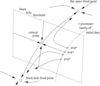
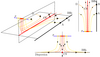
As illustrated in Figures 1 and 2, any trajectory beginning near the critical surface, but not necessarily near the critical point, moves almost parallel to the critical surface towards the critical point. Near the critical point the evolution slows down, and eventually moves away from the critical point in the direction of the growing mode. This is the origin of universality. All details of the initial data have been forgotten, except for the distance from the black hole threshold. The closer the initial phase point is to the critical surface, the more the solution curve approaches the critical point, and the longer it will remain close to it. We should stress that this phase picture is extremely simplified. Some of the problems associated with this simplification are discussed in Section 2.5.

Figure 1: The phase space picture for the black hole threshold in the presence of a critical point. Every point correspond to an initial data set, that is, a 3-metric, extrinsic curvature, and matter fields. (In type II critical collapse these are only up to scale). The arrow lines are solution curves, corresponding to spacetimes, but the critical solution, which is stationary (type I) or self-similar (type II) is represented by a point. The line without an arrow is not a time evolution, but a 1-parameter family of initial data that crosses the black hole threshold at p = p_*. The 2-dimensional plane represents an (–1)-dimensional hypersurface, but the third dimension represents really only one dimension.

Figure 2: A different phase space picture, specifically for type II critical collapse, and two 2-dimensional projections of the same picture. In contrast with Figure 1, one dimension of the two representing the (infinitely many) decaying modes has been suppressed. The additional axis now represents a global scale which was suppressed in Figure 1, so that the scale-invariant critical solution CS is now represented as a straight line (in red). Several members of a family of initial conditions (in blue) are attracted by the critical solution and then depart from it towards black hole formation (A or B) or dispersion (D). Perfectly fine-tuned initial data asymptote to the critical solution with decreasing scale. Initial conditions starting closer to perfect fine tuning produce smaller black holes, such that the parameter along the line of black hole end states is –ln M_BH. Two 2-dimensional projections of the same picture are also given. The horizontal projection of this figure is the same as the vertical projection of Figure 1.

"Critical Phenomena in Gravitational Collapse" Carsten Gundlach and José M. Martín-García http://www.livingreviews.org/lrr-2007-5

This work is licensed under a Creative Commons License. Problems/comments to