2.1 Overview of gravity Feynman rules 

Scattering of gravitons in flat space may be described using Feynman diagrams [44, 45, 138]. The Feynman rules for constructing the diagrams are obtained from the Einstein-Hilbert Lagrangian coupled to matter using standard procedures of quantum field theory. (The reader may consult any of the textbooks on quantum field theory [107, 141] for a derivation of the Feynman rules starting from a given Lagrangian.) For a good source describing the Feynman rules of gravity, the reader may consult the classic lectures of Veltman [138].

  

Figure 1: The Feynman propagator and three- and four-point vertices in Einstein gravity.

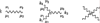
The momentum-space Feynman rules are expressed in terms of vertices and propagators as depicted in Fig.  1 . In the figure, space-time indices are denoted by and while the momenta are denoted by k or . In contrast to gauge theory, gravity has an infinite set of ever more complicated interaction vertices; the three- and four-point ones are displayed in the figure. The diagrams for describing scattering of gravitons from each other are built out of these propagators and vertices. Other particles can be included in this framework by adding new propagators and vertices associated with each particle type. (For the case of fermions coupled to gravity the Lagrangian needs to be expressed in terms of the vierbein instead of the metric before the Feynman rules can be constructed.)

According to the Feynman rules, each leg or vertex represents a specific algebraic expression depending on the choice of field variables and gauges. For example, the graviton Feynman propagator in the commonly used de Donder gauge is:

 

The three-vertex is much more complicated and the expressions may be found in DeWitt's articles [44, 45] or in Veltman's lectures [138]. For simplicity, only a few of the terms of the three-vertex are displayed:

 

where the indices associated with each graviton are depicted in the three-vertex of Fig.  1, i.e., the two indices of graviton i = 1, 2, 3 are .

  

Figure 2: Sample gravity tree-level Feynman diagrams. The lines represent any particles in a gravity theory.

  

Figure 3: Sample loop-level Feynman diagrams. Each additional loop represents an extra power of Planck's constant.

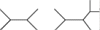
The loop expansion of Feynman diagrams provide a systematic quantum mechanical expansion in Planck's constant . The tree-level diagrams such as those in Fig.  2 are interpreted as (semi)classical scattering processes while the diagrams with loops are the true quantum mechanical effects: Each loop carries with it a power of . According to the Feynman rules, each loop represents an integral over the momenta of the intermediate particles. The behavior of these loop integrals is the key for understanding the divergences of quantum gravity.

Perturbative Quantum Gravity and its Relation to Gauge Theory Zvi Bern http://www.livingreviews.org/lrr-2002-5 © Max-Planck-Gesellschaft. ISSN 1433-8351 Problems/Comments to livrev@aei-potsdam.mpg.de